Figure 1. Visualization of the CIFAR10 embedding (on the left) vs. the core, i.e., the innermost layer on right
Characterizing and exploiting density–geometry correlations in high-dimensional data
Density-geometry correlations in high dimensional data.
Density and geometry have been two fundamental aspects of algorithm design in unsupervised learning. For example, in clustering, algorithms like GMM and density-peak clustering aim to find clusters by detecting high-density regions whereas manifold clustering algorithms assume data from different clusters lie in separate low dimensional manifolds.
In our recent works (in [1] and other works in progress), we have observed a very interesting density-geometry interaction in a wide variety of datasets. Specifically we observe that in problems where data is embedded on a vector space and is expected to have some underlying ground-truth partitioning into groups or types (cluster), the following happens.
Each underlying cluster contains a high-density low-complexity region that is well-separated from other clusters
As we move away from these higher density regions, i) Density goes down. ii) The complexity of the space goes up (more on this later as well)
We observe these phenomena in
1) Almost all standard image datasets (such as MNIST, Fashion-MNIST, CIFAR10, CIFAR100) both in their standard vectorized form as well as deep learning based embeddings such as from CLIP.
2) A wide varity of single-cell RNA-seq datasets, one of the most influential modalities of genomics data of the last decade.In this direction, we present a theoretical model of the data and an algorithmic framework built on it that captures and exploits the aforementioned characteristics, leading to
A novel perspective on capturing stable-transcriptomic states in complex single-cell RNA-seq datasets, that allows robust cell-type identification as well as identification of novel stable and transient cell states that can be missed by existing frameworks.
A clustering enhancement framework
a) That improves the performance of K-Means on image datasets, making it competitive with state-of-the-art manifold clustering algorithms. b) Massively improves non-parametric clustering algorithms such as HDBSCAN.A novel CNN-based semi-supervised learning algorithm that outperforms the SOTA (such as Flexmatch and Freematch) significantly across a large set of image datasets and for different label-per-class settings.
The LCPDM Model:
Now, we briefly explain our model (a detailed explanation can be found in [1]).
We assume points of each ground-truth cluster \(i\) are generated from some \(\mathcal{X}_i \subseteq \mathbb{R}^d\), where all the points lie on some \(m\)-dimensional smooth manifold \(\mathcal{M}\).
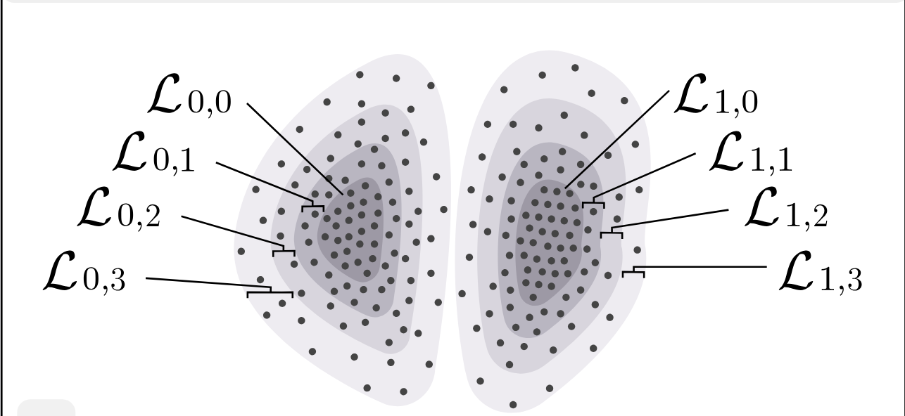
Concentric subspaces. The fundamental assumption we make is that \(\mathcal{X}_i\) can be expressed as a hierarchy of concentric subspaces \[ \mathcal{X}_{i,0} \subset \mathcal{X}_{i,1} \subset \cdots \subset \mathcal{X}_{i,\ell-2} \subset \mathcal{X}_{i,\ell-1} = \mathcal{X}_i. \]
We call the difference between the \(j\)-th and \((j+1)\)-th subspace the \(j\)-th layer \(\mathcal{L}_{i,j}\), defined as \[ \mathcal{L}_{i,0} := \mathcal{X}_{i,0}, \qquad \mathcal{L}_{i,j} := \mathcal{X}_{i,j} \setminus \mathcal{X}_{i,j-1}, \quad 1 \le j < \ell. \]
Each \(\mathcal{L}_{i,j}\) is smooth and has a minimum and maximum depth in any direction. We call \(\mathcal{L}_{i,0}\) the core and the outer layers peripheral. We assume each layer is connected and has finite volume in a well-defined measure.
We collectively term these assumptions the Layered-Core-Periphery-Density Model (\(\mathsf{LCPDM}\)). The figure below provides a schematic representation.
The Layered-Core-Periphery-Density Model \({\sf LCPDM}(k,\ell)\)
Cores are dense and peripheries are sparse. The data is generated by sampling \(n_{i,j}\) points from each layer \(\mathcal{L}_{i,j}\) uniformly at random, such that there exists a constant \(C>1\) satisfying \[ \frac{n_{i,j}}{\mathrm{Vol}(\mathcal{L}_{i,j})} > C \cdot \frac{n_{i,j+1}}{\mathrm{Vol}(\mathcal{L}_{i,j+1})}. \]
That is, the inner-most layer (the core) is densest, and outer layers are progressively sparser. We denote points from \(\mathcal{L}_{i,j}\) as \(\widehat{\mathcal{L}}_{i,j}\).
Cores are well-separated. The cores of clusters are well separated in Euclidean space. For any clusters \(i,i'\), \[ \exists\, \mu_{i,i'} < 0.5 \text{ such that } \max_{\substack{\mathbf{x} \in \widehat{\mathcal{L}}_{i,0}\\ \mathbf{x}' \in \widehat{\mathcal{L}}_{i,0}}} \|\mathbf{x}-\mathbf{x}'\| \;\le\; \mu_{i,i'}\! \cdot \min_{\substack{\mathbf{x} \in \widehat{\mathcal{L}}_{i,0}\\ \mathbf{x}' \in \widehat{\mathcal{L}}_{i',0}}} \|\mathbf{x}-\mathbf{x}'\|. \] For two clusters, define \(\mu := \mu_{0,1}\).
Identity of points in outer layers: The group identity of the points in the outer layer is more context dependent. In some cases, every point in the dataset can be attributed to having some ground truth labels (such as the standard image datasets CIFAR), and in some cases the outer labels may not have any “true” labels (as we shall observe for scRNA datasets).
The core-extraction procedure:
First, we describe a framework to extract the core (the innermost layers) of different regions of the data, followed by usefulness of said method.
Observing UMAP of whole data vs. core for hard-to-separate clip embedding:
The LCPDM structure in CIFAR10 embedding:
Figure 2. The LCPDM structure in CIFAR10 embedding
As we can see, the cores look much easier to separate compared to the rest of the data. In the next part, we will observe that these cores have some desirable properties when analyzing single-cell RNA-seq datasets.
Robust cell-type identification in scRNA data via recovery of stable-transcriptomic states:
In a work in progress, we are currently working on a single-cell RNA-seq analysis pipeline (https://github.com/CrossOmics/scRNA-seq), where our first step is to extract the underlying core-to-periphery layers in a given dataset. We give some evidence of how these layers can be used for more robust and principled inference of scRNA data.
Stable transcriptomic states:
In the analysis of sc-RNA seq data, one of the most popular pipeline is
Pre-processing ⟶ Clustering ⟶ Detect upregulated or downregulated genes in each clusterIf the scRNA data has meaningful boundaries w.r.t. cells with different functionalities, this method can lead to uncovering of important biological information, such as genes associated with specific phenomena or disease. This behavior has led to several discoveries using scRNA datasets.
However, in more complex datasets there may not be any clean separation between cells with different functionalities, and as such, clustering of the whole dataset may lead to irreproducible and/or noisy outcome. Consider the following dataset from [2] that containing subtypes of Natural killer cells.
We run the popular single-cell analysis scanpy [3] algorithm on this dataset with resolution 1.5 several times to get labels, and present the UMAP for three runs here:
Figure 3. Visualization of two independent runs of scanpy on the NK-cells dataset
As one can observe, the labels in the middle of the dataset changes significantly across runs. In fact, the average ARI between the labels output by different runs is only around 0.6 indicating a high instability.
In comparison, the core extracted by our method (with labels obtained with scanpy) is as follows:
The NK-cell dataset through the lens of layer-extraction:
Figure 4. Layer extraction and clustering on the NK-cell dataset.
As we can observe, we still recover the same number of clusters, but the boundary separation is very obvious, and across multiple runs, the ARI between labels are now 0.98!, this indicates that scanpy’s behavior is reproducible on the cores even if the performance on the overall dataset is unstable. Here we have two more promising directions.
We observe that our clusters match the DEG profiles obtained by applying scanpy on the whole dataset, but the cores have significantly stronger signals (for several important upregulated and downregulated genes). This indicates that the cores we find are some sort of “transcriptomically stable” states, with stronger signal and clear boundary separation from other states. We are in the process of verifying this thoroughly for multiple datasets.
Once we have this stable states, different intermediate states can also be captured by looking at the cells from outer layers that reside between different stable states. We are currently exploring this direction.
Extending labeling to the rest of the data: A clustering enhancement framework:
Based on [1]. This will be expanded on shortly.Semi-supervised learning through the lens of density-geometry correlations:
Based on joint work with Nikhil Deorkar. This will be expanded on shortly.References:
[1] Mukherjee, Chandra Sekhar, Joonyoung Bae, and Jiapeng Zhang. “CoreSPECT: Enhancing Clustering Algorithms via an Interplay of Density and Geometry.” arXiv preprint arXiv:2507.08243 (2025).
[2] Rebuffet, Lucas, et al. “High-dimensional single-cell analysis of human natural killer cell heterogeneity.” Nature immunology 25.8 (2024): 1474-1488.
[3] Wolf, F. Alexander, Philipp Angerer, and Fabian J. Theis. “SCANPY: large-scale single-cell gene expression data analysis.” Genome biology 19.1 (2018): 15.